Destructible Large-Scale Voxel Planets using Surface Nets
A while back, I showed my first implementation of a Smooth Voxel Terrain. While I was reasonably satisfied, it left a lot to be desired. The terrain suffered from some artifacts and performance issues, and because it was programmed in C# it could not be easily integrated into other projects. For these reasons, I decided to start working on a new implementation from scratch in C++, addressing many of these problems. While the new version is not production ready by any means, feel free to check out the source code here. This newer implementation has a greater focus on spherical planets, but should work for any kind of terrain.
Terrain Structure & Data
First, I will provide an overview of the voxel terrain system. As it shares many similarities with the previous one, please skip ahead If you’re more interested in the meshing stage of the algorithm.
Just like the previous version, the terrain is a realization of the implicit surface created by a signed distance field, or SDF. SDFs are functions that return the distance from a point to the surface, positive if considered outside, and negative if inside. SDFs are known for many basic functions, such as spheres, planes and cubes. But they can represent virtually any geometry by combining multiple SDFs using boolean operations.
Depending on the SDF, it can be expensive to evaluate. To reduce computations every time the terrain updates, I store SDF values as voxel data in a data structure, so the CPU can read the values from memory instead. This simplifies implementing real time modifications too. We can now directly edit the stored values, rather than having to combine many SDF functions. This in turn means that players can dig or add to the terrain with ease.
In our case, this data structure is an octree. It’s essentially a binary tree in 3D, as it subdivides each axis per layer, resulting in 8 children per node. We commonly use an octree precisely because it’s so effective at partitioning a 3D world. Unlike a uniform grid, an octree can easily allocate more memory to important parts. Homogenous volumes, such as parts that are fully air or fully solid don’t need to be stored at the highest resolution. Instead, we can program our octree to only subdivide if it contains an SDF surface within it. This way, we can generate gigantic worlds without completely filling up the memory of our system.
An octree also inherently lends itself well to implementing level of detail, or LOD. This commonly refers to using lower resolution objects further from the camera. If you go one layer up in the octree, you effectively cut the resolution in half. By storing SDF values not only in the leaves, but also in each inner node, we can take nodes from any particular level of detail, and use those to create a mesh with the desired quality. Thus, the octree not only stores voxel data spatially, but it also provides a hierarchy of increasingly higher resolution representations of the world, at the cost of higher but manageable memory use.
Terrain Meshing System
Now we have all this volumetric data representing our terrain, efficiently stored in an octree. It’s not too useful on its own, so we need to convert it into a mesh. To achieve this, we can use an isosurface extraction algorithm, such as surface nets.
The basic surface nets algorithm has two stages. In the first stage, it collects groups of 8 neighbouring nodes, and places a vertex based on the voxel values. In the second stage, it connects neighbouring vertices by adding quads for every edge between nodes that intersects the implicit surface. Either way, it is clear that the algorithm relies on getting neighbouring voxels. In the octree, we would rely on constant binary searches to find neighbours, which is fast, but we can do it faster. So instead, I collect all nodes in a chunk, and write them into a grid lookup table. This enables us to find neighbours in constant time during the surface nets algorithm, with minor overhead. I won’t go into much more detail about basic surface nets. Instead, I will focus on other challenges related to LOD in this context. Please refer to my previous post for more details.
Chunks & LOD
While extracting a surface works great, one large mesh is wasteful if we want to modify a part of the terrain, as we would have to recompute the entire mesh. Moreover, you cannot frustum cull parts of the terrain this way. Therefore we use chunks, or meshes that span a unique small section of the world. Each chunk can also represent a part of the world in a particular level of detail. By doubling a chunk’s size every time its level of detail decreases, we keep the workload to compute a chunk’s mesh the same regardless of LOD.
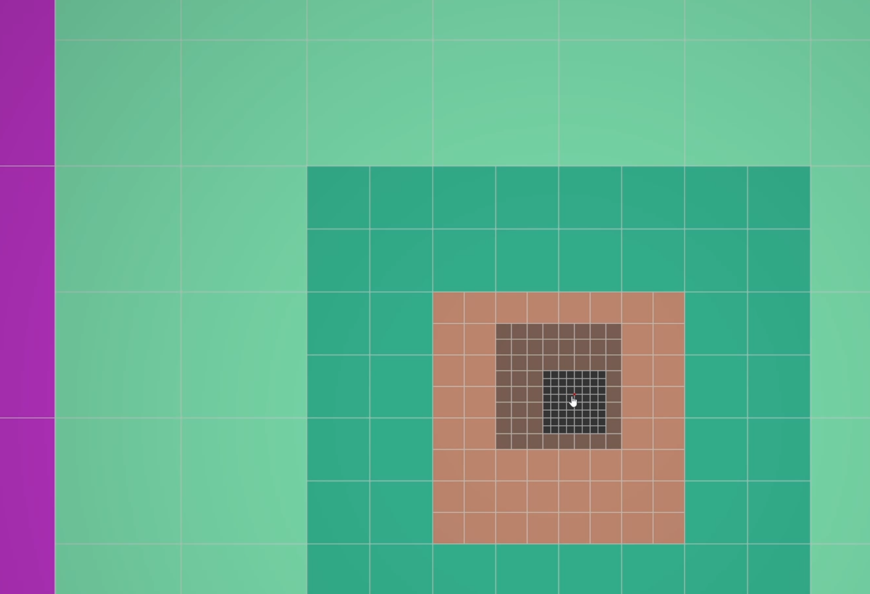
It’s actually not too trivial to compute the desired level of detail of a chunk, given its position relative to the camera. The problem is that we want to compute a level of detail, based on the logarithm of the L-infinity norm of the difference between a position and the reference lod center, but in such a way that the computed values are aligned to the grid such that all nodes in a chunk have uniform LOD.
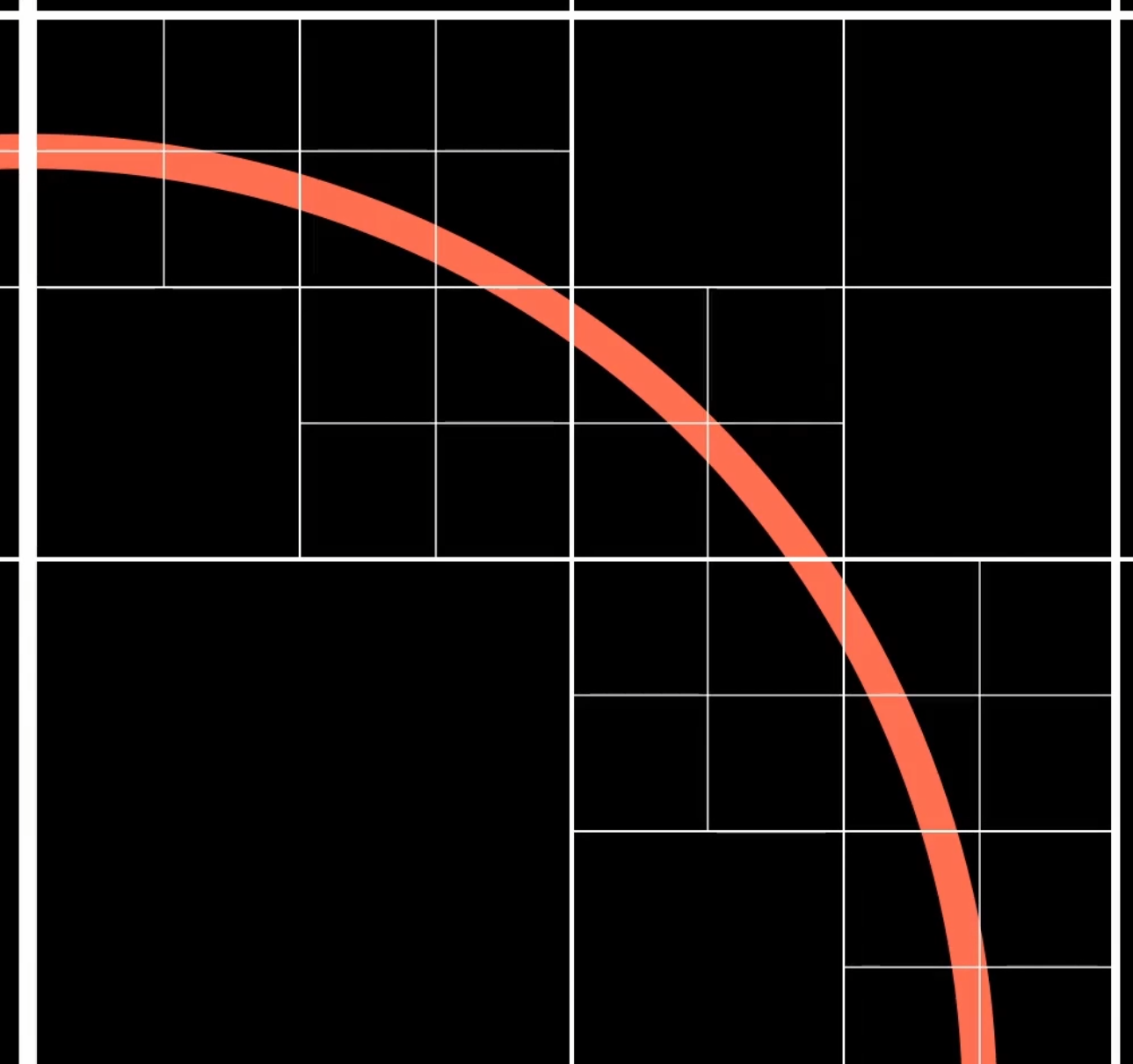
$$ \text{LOD}(p, c) = \left\lceil \log_{2}\left( \max\left(1, \frac{|p-c|_{\infty}}{2*,\text{SHELL_RADIUS}}\right) \right)\right\rceil$$
In other words, we want to compute these recursive shells that are aligned with a grid that itself decreases in resolution as LOD decreases. One way to do this, is to compute the approximate LOD first, and then we can correct by checking if it falls in the computed lod’s shell, or the one below. To play around with this, check-out my demo on shadertoy
However, now that we have split the world into chunks, and ones of varying LODs at that, we introduced a major issue. Chunks are not connected to each other! If we look at it in 2D, we notice that each chunk is 16 by 16. As surface nets is a dual approach, we get a vertex grid of 15 by 15. To tile the world seamlessly, we need a grid of 16 by 16 quads per chunk. That requires 17 by 17 vertices! The chunk meshes need to have the exact same vertices at chunk boundaries to make the world appear seamless. This is quite easy to achieve for chunks of the same level of detail, as we can fetch all nodes in a ring around the chunk too. This way, we recompute vertices on chunk borders twice, one for each chunk mesh they belong to. Luckily, that is not very expensive.
Connecting chunks of different LOD
This becomes a more difficult problem when we consider neighbouring chunks of differing LOD. For the previous implementation, I proposed to use a higher resolution grid to facilitate nodes from different LODs next to each other. However, I noticed some terrible artifacts in the normals on LOD boundaries, and the implementation in general felt convoluted.
Therefore, I began working on another implementation. Some voxel meshing algorithms stitch chunks together, by connecting vertices on the edges of chunks with new quads. I am not a big proponent of this approach, as it introduces a dependency on neighbouring meshes. In my opinion, it is best if each chunk mesh is independent of all neighbours, instead only depending on the voxel state in the octree. That way, we can clearly separate the updating octree stage, and the meshing stage, into two individual processes.
So instead, we take the best of both worlds. Much like with chunks of identical LOD, we want to take in extra data to compute vertices on the boundaries between chunks. We take a 2 by 8 by 8 slice of the lower LOD nodes for each chunk boundary from high LOD to low LOD. I refer to these nodes as ring nodes. The reason we only consider the boundary from high to low, is because this only requires us to look in 6 directions, rather than 27. Then, for each collected ring node, we compute vertices as normal. Importantly, we store these ring nodes in a hashmap that maps an integer 3d position to a node. We also store all regular nodes on the boundary of a chunk in a different hashmap. It’s important that these hashmaps are different, as they require different resolutions. We don’t want holes in our lookup table, and the ring nodes are twice as big, thus half as frequent. Therefore, we index into the ring hashmap using coordinates that are divided by two, relative to the inner node hashmap.
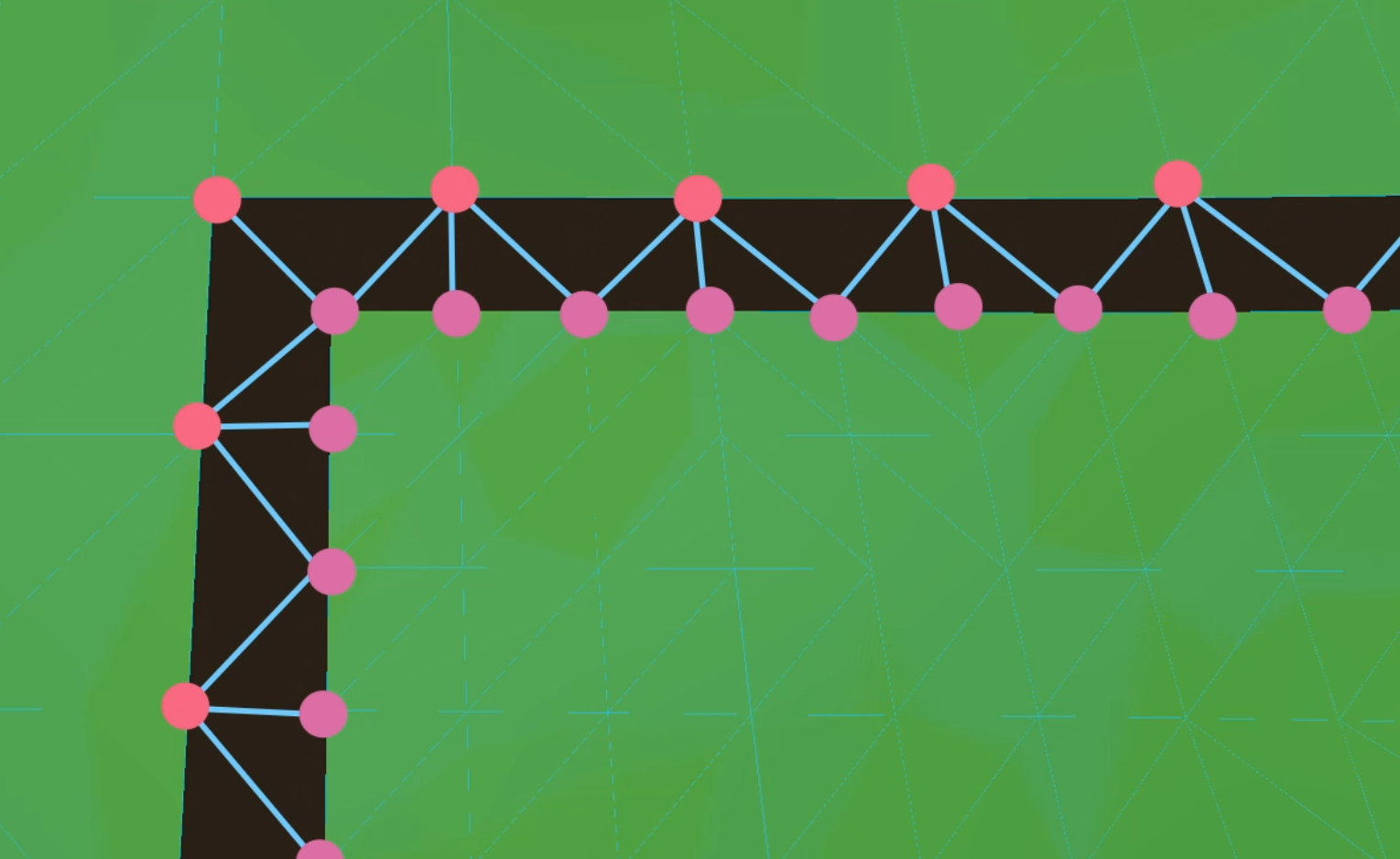
Once collected, we want to connect the regular boundary nodes and the ring nodes. We do this by iterating over the regular boundary nodes, and finding another neighbouring regular boundary node. If successful, we try to find one or two ring neighbours, and make a triangle or quad respectively.
Because vertices are always computed the same way, the connection between chunks looks rather satisfactory now. The implementation is not strict enough, so there is some limited additional overdraw, but I don’t see this as a huge issue for the time being.
Overall, I am much happier with this implementation. As of right now, I am unsure of my future plans, but I’m considering implementing some more features. For instance, I am not happy with the way colliders are generated. Godot handles this on the main thread, which causes major frame spikes. The terrain system will require much more work to become production ready, so consider using alternatives like Zylann’s amazing voxel engine instead. Of course, I have open sourced this project under the MIT licence, so feel free to use it in any way you like.