Large-Scale Smooth Voxel Terrain
Update:
I rewrote this project from the ground up in C++, and I made some algorithmic improvements. Please refer to the new version.
Rendering large terrains is no easy task. In real-time computer graphics, terrains are often large subdivided planes with vertices translated vertically based on a heightmap, but this means that overhangs or caves are impossible without extra work or additional meshes. Instead, we can use a three dimensional volume to represent the terrain. However, if we want a 4 by 4 by 4 kilometer 3D terrain at a 1 cubic meter resolution with just a floating point number at every position, we would need about a quarter terabyte of memory. I have therefore set out to create an efficient system that generates a smooth and watertight triangle mesh terrain, based on a voxel octree. I chose to implement it in Godot using the c# programming language. To understand the implementation, we first need to go over some concepts.
Heightmaps and Signed Distance Fields (SDFs)
In computer graphics, a terrain is a large surface, often represented using a triangle mesh. We can use a heightmap or a function that returns a height value for each horizontal position and apply it to the vertices of a subdivided plane to get something representing a terrain:
However, heightmaps provide only one height value per horizontal position. If we want overhangs, caves, or the ability to freely edit the terrain, we instead need a function that somehow defines a surface for any three-dimensional position:
$$F(x,y,z) \rightarrow ?$$
Signed distance fields, or SDFs do just that. These are functions that return the signed distance from a point in space to an implicit surface. The implicit surface is the set of all points whose function values equal zero:
$$ (x, y, z) \in \mathbb{R}^3 \mid f(x, y, z) = 0 $$
SDFs are known for many primitive shapes, such as spheres, planes and cubes. Signed distance refers to distance values that may be negative. When distance is negative, it’s inside the volume enclosed by the implicit surface. Conversely, when the distance value is positive, it’s outside the volume. Multiple SDFs can be combined using boolean operations, such as union and difference.
Isosurface Extraction using Surface Nets
SDFs are not useful on their own, we need to somehow render them onto the screen. A common technique is raymarching, which is essentially a form of raytracing. Alternatively, isosurface extraction can be used, which are algorithms that aim to generate a polygonal mesh that best approximates the SDF’s implicit surface. While the marching cubes algorithm is the most common for this task, I chose to implement surface nets because it is better suited to mesh between chunks of different levels of detail, and fast surface nets implementation exist.
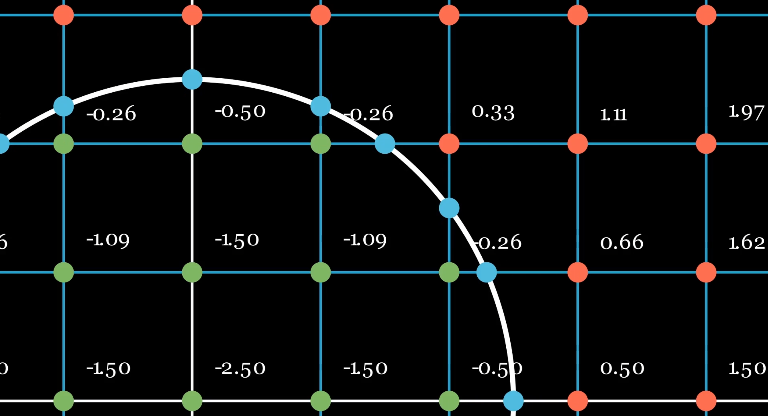
The surface nets algorithm works as follows: Firstly, we sample SDF values in a voxel grid. Secondly, we calculate intersections of the SDF surface with each grid line. We can do this by iterating through all twelve edges of a particular cubical node, and checking if the sign between the values of the two ends of the edge A and B is different. If so, we calculate the point of intersection (PoI) using:
$$t = \frac{|Value_A|}{|Value_A| + |Value_B|}$$
$$ PoI = Position_A * (1 - t) + Position_B * t$$
Next, for each cell, we average the edge intersection positions for each edge around it to get a single vertex position per cell. Finally, for each edge that intersects the implicit surface, we add a quad between the vertices of the four cells that share this edge. We are now left with a mesh that resembles the original implicit surface. We need to ensure that the triangles in the quad are wound such that the normal would point in the direction of positive increase in the SDF. We manage this by changing the winding order based on which vertex in the edge through the quad is negative.
To achieve smooth shading, we want to calculate a normal for each vertex based on the SDF. The goal is that we have a normal that points in the direction of the largest gradient in the original SDF. We can approximate it using:
$$ normal = \frac{1}{|E|} \sum_{A,B \in E} (( \text{value}_B - \text{value}_A ) \cdot \frac{\text{pos}_B - \text{pos}_A }{||\text{pos}_B - \text{pos}_A||})$$
Here E is the set of all cube edges that intersect the implicit surface.
This seems ineffective in cases where chunks of two different levels of detail meet. Instead, we can calculate the normal by fitting a plane to the set of points of intersections (PoIs) calculated earlier.
Here is the C# code I use for it:
        public static Vector3 Fit(List<Vector3> points, Vector3 centroid)
        {
            var covariance = CovarianceMatrix(points, centroid);
            var evd = covariance.Evd();
            var smallestIndex = evd.EigenValues.AbsoluteMinimumIndex();
            var normal = evd.EigenVectors.Column(smallestIndex);

            return new Vector3(normal[0], normal[1], normal[2]);
        }
Scalability and Level of Detail (LoD)
While this works great, we are left with the problem of scalability. In real-time rendering this is often addressed using various Levels of Detail, or LOD techniques. If we want to compute and render large terrain in a time and space efficient manner, we need to render further geometry at a lower resolution. A data structure that facilitates this for voxel data is an Octree. It is a tree made up of nodes with either eight or zero children each. This type of tree divides the 3D volume of a node into smaller sections, allowing for faster processing and less memory usage by undersampling homogenous areas far from the implicit surface, or far from the camera. This means we will not represent the SDF fully accurately in the octree, but the resolution will always be high near the implicit surface, which is important for isosurface extraction.
We can build the tree based on two principles: We subdivide a node if both the SDF evaluated at its center is smaller than the distance to its center and a corner, and a node is close to the camera. The evaluated SDF value is then stored in the node. The advantages over a uniform grid are thus twofold: SDF samples are only stored densely close to the implicit surface, and sample density decreases as the distance to the camera increases.
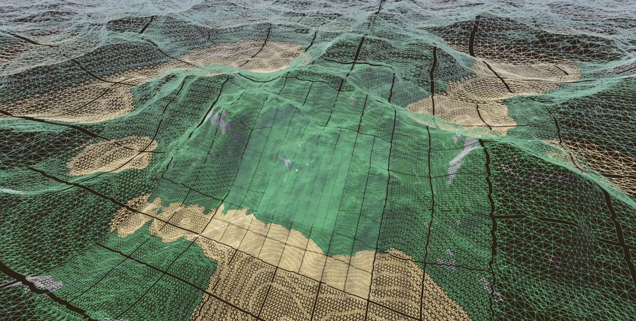
To improve performance, we want to cull parts of the terrain that are not on screen. And when editing a piece of terrain, we want to only regenerate parts of the terrain close to where it is edited. To facilitate this, we divide the terrain up into chunks. We can directly use the octree for this. A node is considered a chunk if its n sizes above the level of detail at its position, where I choose n = 4, resulting in 16x16x16 nodes per chunk. Chunks further away are also bigger in size, but equal in relative triangle resolution. This uses fewer objects and draw calls to render the terrain compared to an approach where chunk sizes are static.
However, chunks also have a downside. To make a tight mesh, we need information from neighboring chunks. A tight mesh would require n faces in a certain dimension, which itself requires n + 1 vertices. As each vertex is calculated using its 7 direct and diagonal positive neighbors, we need n + 1 + 1 nodes per dimension. Therefore we sample one extra node from neighboring chunks in all directions, resulting in a 18×18×18 input to the surface nets algorithm.
Changes to Surface Nets
Surface nets originally requires a uniform voxel grid, not an octree. Luckily, its principles can relatively easily apply to an octree, unlike marching cubes, which relies on a lookup table that expects a uniform voxel grid. (Unless complex add-ons such as Transvoxel are used!)
I came up with several techniques to apply surface nets to an octree. Firstly, I temporarily create a 3D array which stores references to the leaves of the octree within a certain chunk. This means I can get the neighbors of each node in constant time, at the cost of linear time with respect to the leaves at the start of the meshing algorithm.
Secondly, instead of taking the positive neighbors of nodes to calculate vertices, I consider neighbors in the outward direction away from the camera position. This effectively means only transitions from small to large nodes have to be considered, which makes the code simpler, but incompatible with octrees that are not only increasing in node size as distance to the camera increases.
Finally, if an edge is shared by just three nodes, one big node and two small ones, I create a triangle instead of a quad to complete the mesh. This allows us to create a mesh that perfectly connects nodes from different levels of detail.
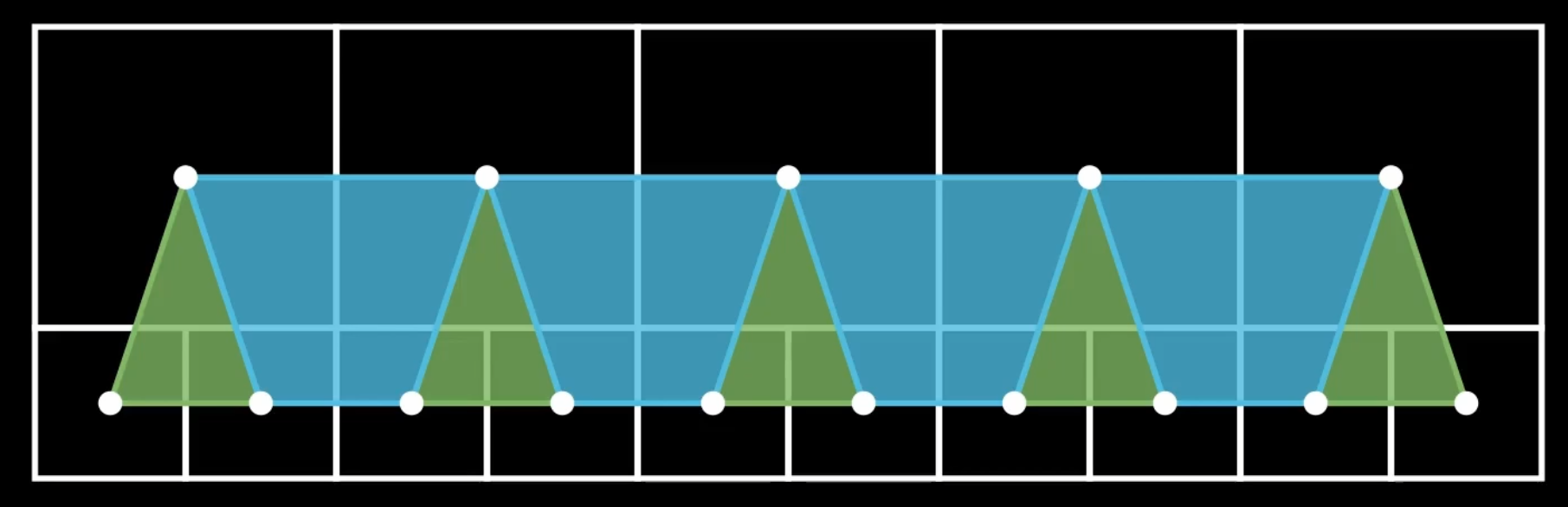
Nodes from different LoDs can still be integrated into surface nets by extending it to draw triangles when needed
Editing the terrain
To edit the terrain, we define an SDF, an operation, and an axis-aligned bounding box (AABB) around the edit. For instance, to add a sphere to the terrain, we would want to define SDF describing this sphere with radius r and position p, we set the operation to Union, and we define an AABB that fits tightly around the sphere.
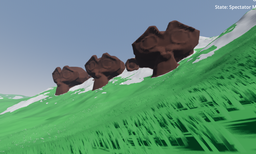
The terrain mesh can be edited relatively efficiently in real-time in two steps. First, we change the octree by finding the leaves that intersect the AABB of the edit operation. The leaves are either pruned if they are fully within the volume of the new SDF, or they can be subdivided if they intersect the new SDF. We calculate a new value for each node by applying the desired boolean operation (Union or Difference) to the node’s current value, and a sample of the new SDF at the node’s center. If the new value and the old value differ by a threshold, I set the red channel of a node’s color to one to mark it as edited.
Next, we remesh all the chunks that intersect the AABB using the updated octree, such that they represent the union of the sphere and the terrain.
Terrain Visuals
Each node in the octree also stores a color. We can set the red channel to one if it has been edited, else zero. During the meshing stage, we calculate the color at Intersection (CaT), just like we calculate the Point of Intersection:
$$ CaT = Color_A * (1 - t) + Color_B * t$$
We average the CaT of all the edges neighboring a node, and set that as the node’s vertex color. Then in the terrain Shader, I currently set the color to brown if the red channel of the vertex color is over 0.5.
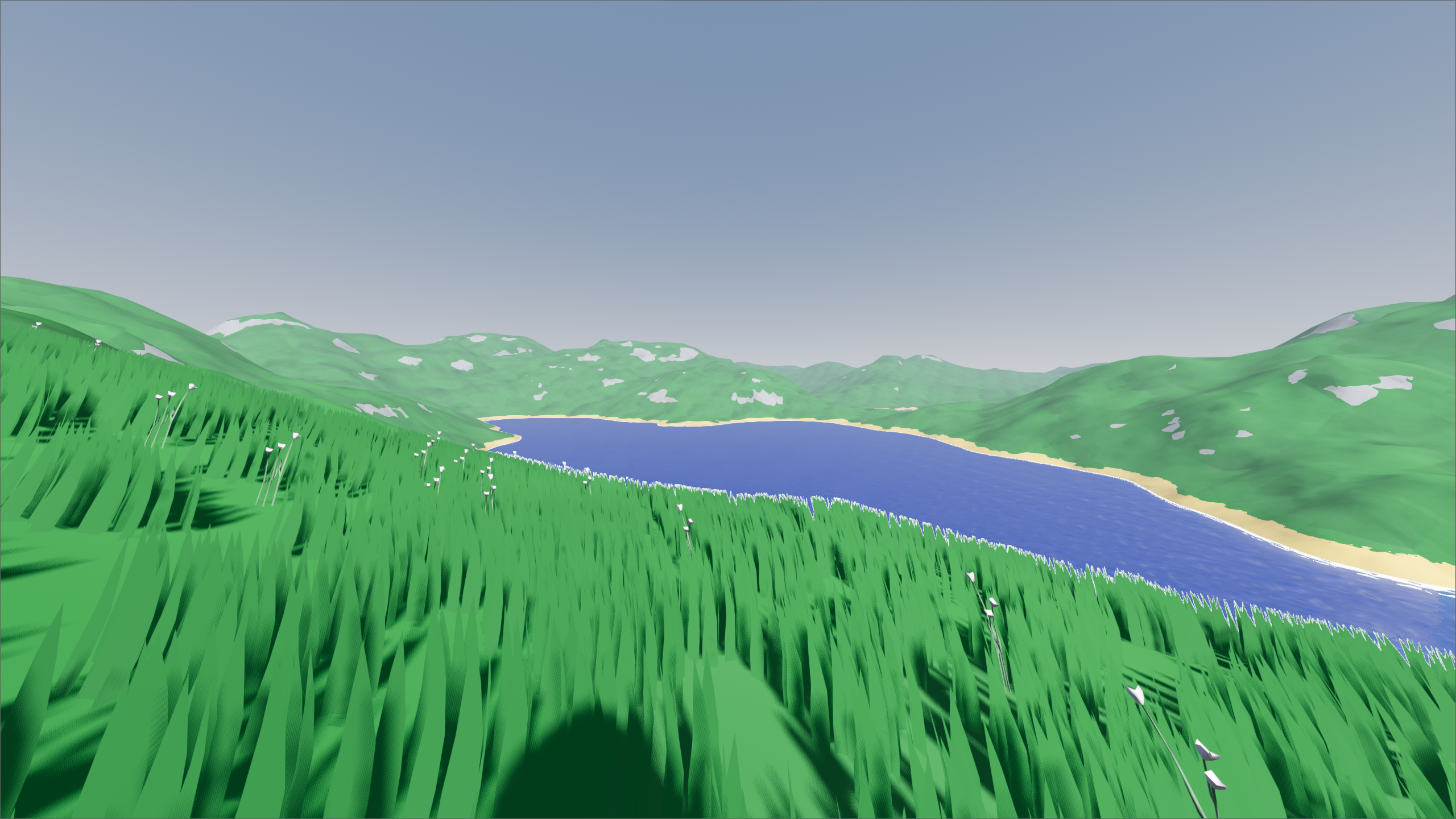
The terrain itself is textured using triplanar mapping, as calculating UVs for these meshes is a hard problem.
Conclusion and Future work
Overall, I believe to have succeeded at creating a fully editable large-scale smooth voxel terrain, with perfect LoD transitions. It generates relatively quickly at an acceptable resolution, perfect for terrains.
There are a number of extensions I am considering for this project. Firstly, I want to be able to populate the terrain with countless objects, such as trees, that can be seen from afar. Secondly, I would like to extend the surface extraction method to guarantee manifold meshes. Thirdly, I would like to optimize the underlying octree structure, to allow for more efficient memory usage, and decrease the time it takes to edit large parts of the terrain.