Ray Marching Fractals that move to Music
I wanted to combine my love for computer graphics and music, by creating a music video generator. The idea is to design a dynamic renderer that enables me to quickly iterate on some neat looking visuals that move to music playing in the background. I realized that one of the best options for this is ray marching, as we can apply many fun tricks to quickly create some sophisticated looking scenes with a bit of mathematics.
For my voxel terrain project, I used signed distance fields or SDFs to describe the surface of the terrain. I visualized the surface by extracting a triangle mesh, and rendering that using rasterization. However, we can also directly visualize the SDFs using ray marching.
Ray Marching
An SDF is a function that describes the distance from a point to some implicit surface. We can easily define these for simple geometric objects such as spheres, boxes and planes. To get more complicated shapes, we can combine them.
To find this surface, we fire a ray from the camera’s position, into the camera’s forward direction. We compute the SDF value d at the current ray step, and we walk d units forward along the ray. We know we will not phase through a surface this way, as our SDF should tell us the minimum distance to any implicit surface at a given position. Ray marching is an iterative approach, and thus we measure the distance again, take another step, and repeat. At a certain point, we will obtain a distance that is under some small threshold value, like 10^-4. At this point we accept that we hit something. If instead we find that the ray is taking too many steps or has exceeded some distance from the ray origin, we discard the ray, and say we missed the scene geometry.
To render an image, we process every pixel individually. The uv coordinate of each pixel in the target image defines a unique ray. We project this coordinate into world space using the view-projection matrix and subtract the camera position to obtain the ray’s direction.
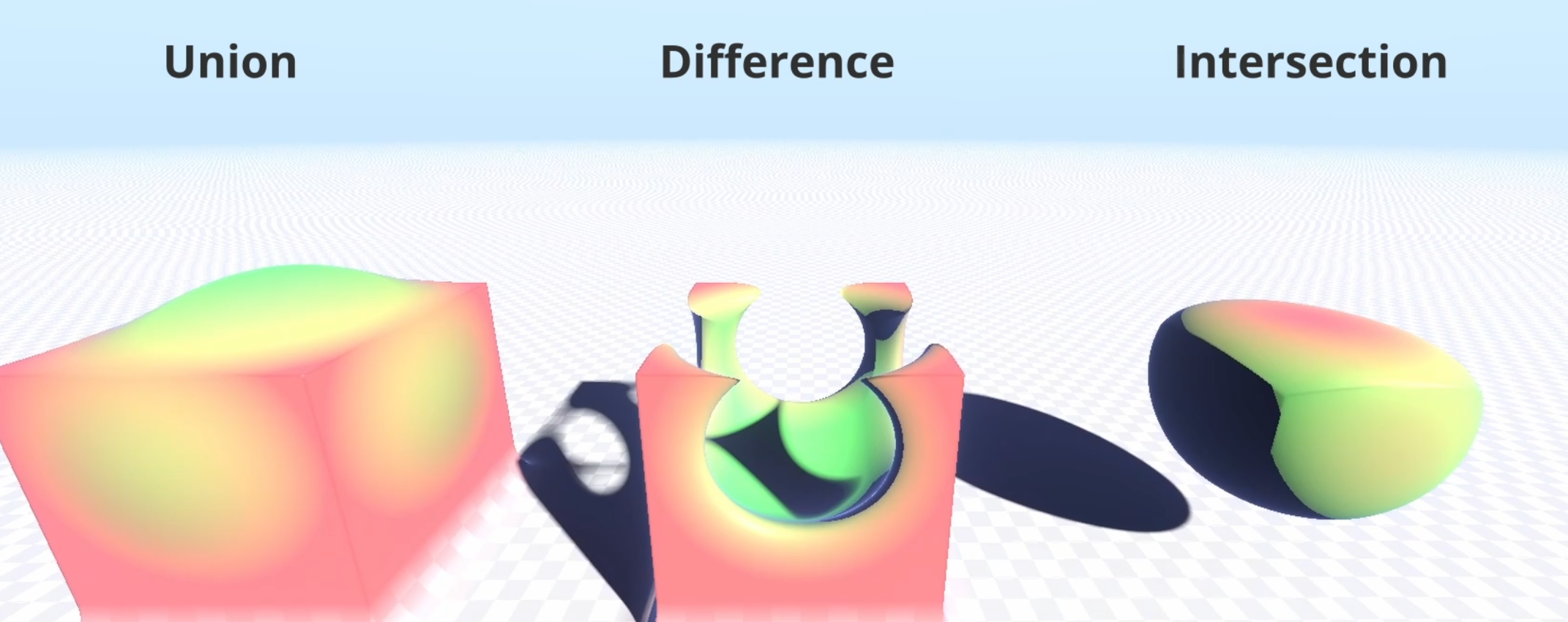
The benefit of SDFs is that they are fully mathematically defined. Instead of creating extra geometry, we can simply repeat the space for free using domain repetition, which is generally done by getting the fractional part of the position. We can also warp or bend the space to get some interesting results. At any point, we can combine SDFs using boolean operators, such as union, intersection and difference. Special versions of these operators exist that smoothly blend between two shapes.
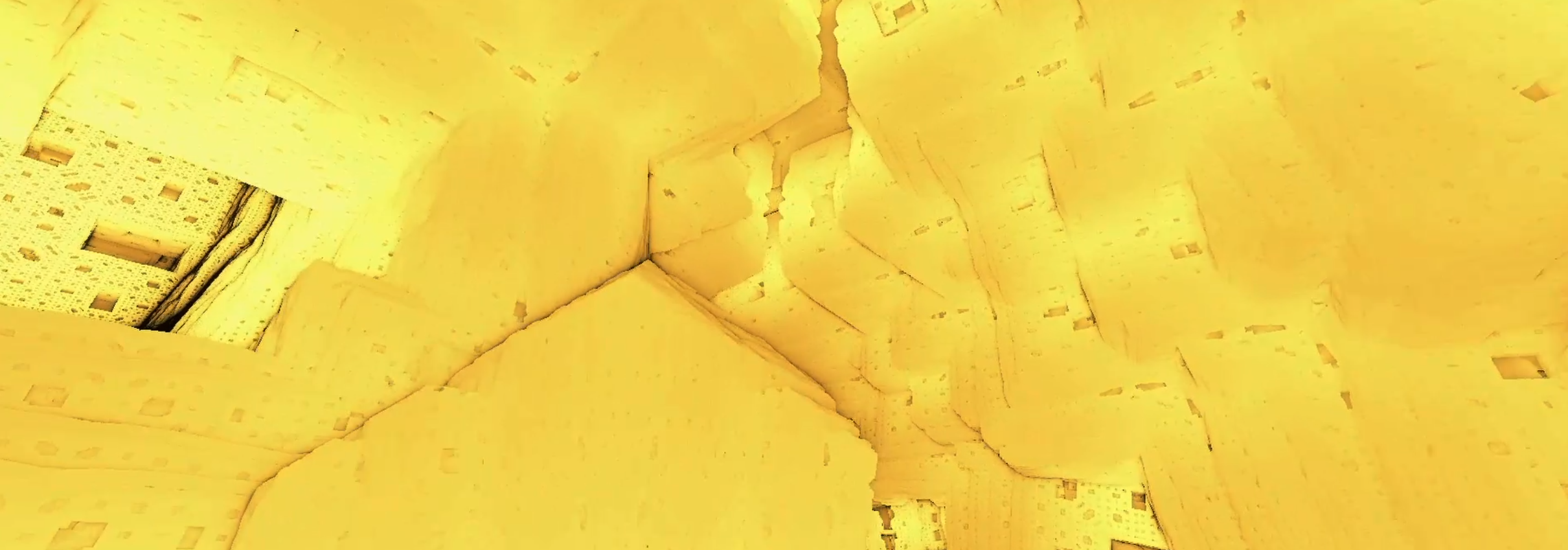
To really get fascinating and intricate results, we can make use of fractals. Fractals emerge from iteratively applying transformations to geometric structures. The Menger Sponge, a well-known 3D fractal, is formed by recursively removing smaller cube-shaped sections from a larger cube. In particular, we use a simple for loop to iteratively carve out a pattern that increases in frequency every iteration. We add some visual interest by transforming the space every iteration, for instance using simple rotation or offsetting.
Lighting effects
A more detailed lighting implementation also improves the quality of our renders. As ray marching is a ray based rendering approach, we can trivially add reflections and shadows by simply casting more rays. If we intersect some geometry, we can compute an approximation of the gradient at the intersection using the central difference method. We use this as the normal of the found surface, and we can reflect the incoming camera ray off of this. We repeat the ray marching step in this direction, and then we simply blend the color of this secondary intersection with the color of the initial geometry. For shadows, we can fire a shadow ray towards each light source, and consider the point to be in shadow if we find an intersection before the light.
Audio Processing
So now we have our dynamic rendering method, but to make the visuals truly responsive, we need to link them to music. We can use scalar variables to control aspects like geometry offsets. But to obtain meaningful values for these variables, we require some signal processing on the music.
A digital audio file consists of two lists of samples—one for the left channel, one for the right. Each sample represents the amplitude of the signal, at a specific point in time. The Nyquist theorem tells us that with a sample rate of around 40 kHz, we can capture frequencies up to 20 kHz, the upper limit of human hearing. By recording thousands of samples per second, we can accurately reconstruct the original sound. To meaningfully visualize the audio, we need to convert our amplitude-based data into frequency-based data. A spectrum visualizer, like those often seen in music videos, shows how different frequency ranges fluctuate in intensity over time—low pitched tones on the left, high tones on the right. To obtain this, we apply the discrete Fourier transform to a section of the digital signal samples around the relevant timestamp, which decomposes it into its frequency components. Beyond rendering a spectrum, we can make the visuals react to specific musical events. A basic approach is expanding elements of the scene when the music is loud, but a more dynamic method involves detecting transients. These are short peaks in loudness when playing a note, like when you pluck a guitar string. These transients appear as sudden spikes in the audio waveform.
To make our scenes properly move to the music, it would thus be interesting to animate them when such a transient is detected, not just when it is loud. One way to do this is to follow the audio signal with two envelopes, one that is slow, and one that is fast. If they differ too much in value, we know that a spike in the audio must have happened, and thus we mark it as a transient.
Additionally, I introduced low-frequency oscillators (LFOs) and beat generators that synchronize with the song, providing an easy way to vary some properties over time. By combining all these techniques, we can create a dynamic scene that effectively moves in sync with the underlying music.
Post Processing
Next up, we can add some post processing to make the scene prettier. In particular, we want to add tone mapping and a glow to the renderer. In Godot, we can handle this using the built-in environment node. Since the renderer uses a compute shader to generate a texture displayed via a TextureRect UI node, the pipeline must be correctly configured. For optimal results, we render in high dynamic range (HDR), allowing colors to go beyond the standard 0-1 range. Instead, we store values in a texture with 32-bit floats per channel. In Godot, enabling HDR 2D and setting the environment’s background mode to “Canvas” ensures proper integration. With this setup, we can apply tone mapping and glow without additional work on our part.
Cone marching
So we’ve now successfully rendered some pretty fractals, but our framerate is a bit low for more complex scenes. SDFs can get quite expensive, with a single evaluation of the function potentially requiring some for loops and expensive expressions such as cross products or the power function. What’s worse, is that for any particular ray, we may have to evaluate the SDF function hundreds of times.
To improve efficiency, we use cone marching, which helps skip unnecessary calculations by computing a safe starting distance for each ray. Instead of processing individual pixels immediately, we first analyze the scene in larger clusters—say, 10×10 pixel groups. By considering a cone originating from the camera and extending through the pixel group boundary, we establish an initial marching distance. As the ray progresses, we halt early if the computed SDF distance falls below the cone’s radius at that point. Continuing beyond this would risk missing smaller details for some of the pixels in the group in the final ray marching pass. This initial estimate is stored in a buffer and passed to the ray marching step, providing a smarter starting point for the algorithm.
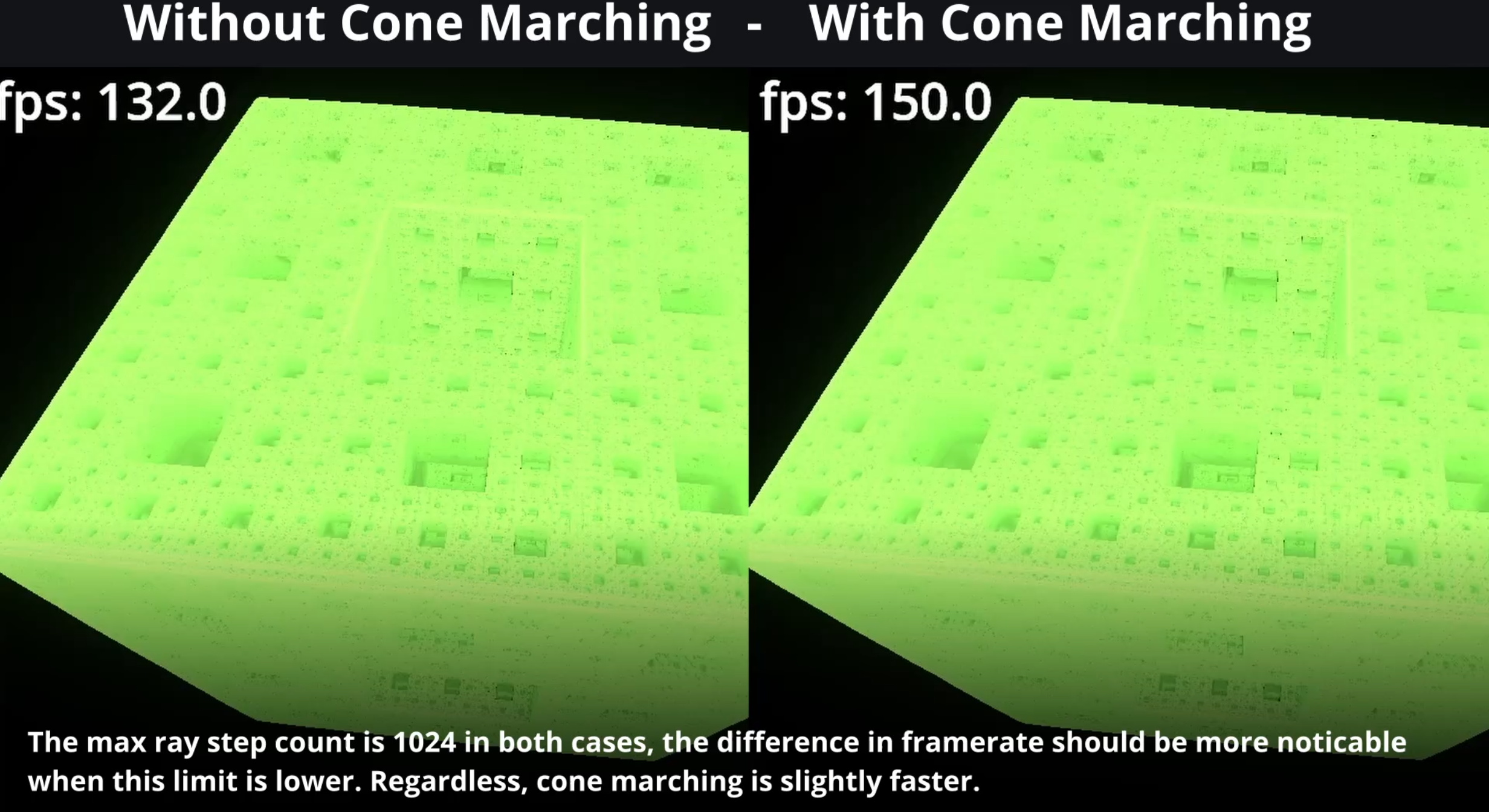
By doing this, we essentially do the first iterations of ray marching 100 times as efficiently, as we effectively consider 100 rays at once. Now the actual performance increase is nowhere near this, as this is unusable for secondary rays, for instance for reflections, and many rays likely have to still travel a fair amount after this minimum distance. Nevertheless, we get a moderate improvement in fps.
Conclusion
Overall, I am happy with the results. I’ve presented a viable framework for making renders that interact with music. I have once again open sourced this project under the MIT license. In the future I may expand it with more scenes or render features.